pygamma cosy

An example of simulating a 2D cosy experiment using pygamma. The example is translated from the original C++ code and the 2D plot is displayed in absolute mode

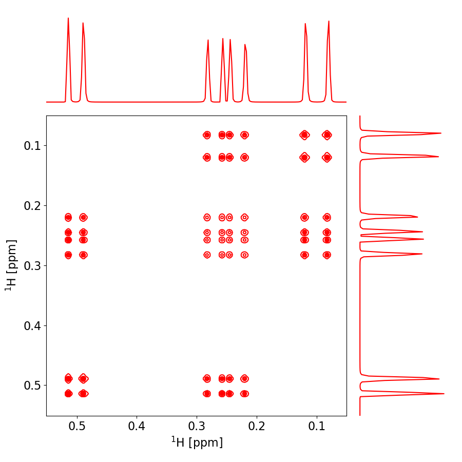
Out:

C:\Users\ERIC\Documents\pygamma_gallery\docsource\sphinx\examples\pygamma_cosy\plot_cosy1.py:162: UserWarning: This figure includes Axes that are not compatible with tight_layout, so results might be incorrect.
  plt.tight_layout()
C:\Users\ERIC\Documents\pygamma_gallery\docsource\sphinx\examples\pygamma_cosy\plot_cosy1.py:241: UserWarning: Matplotlib is currently using agg, which is a non-GUI backend, so cannot show the figure.
  plt.show()

#import pygamma
from pygamma import spin_system, Hcs, HJw, Fm, gen_op, sigma_eq, Iypuls, evolve, FID, row_vector

#import nmrglue

import numpy as np
from scipy import fftpack

import matplotlib.pyplot as plt
from matplotlib.ticker import NullFormatter

class TwoD_NMR_MAT_plot:

    def __init__(self, exp, pinfo, info, dimensions_ppm=[]):

#        print exp.shape

        self.exp = exp
        self.pinfo = pinfo
        self.info  = info

        self.rr,self.cc = exp.shape
        self.X = np.zeros(exp.shape)
        self.Y = np.zeros(exp.shape)

#        r1=0
#        r2=self.rr
#
#        c1=0
#        c2=self.cc

#        print r2,c2

        self.create_axes(  pinfo, info, self.rr, self.cc, dimensions_ppm )

        self.create_plot_layout(self.dimensions_index)

        self.plot_plots()



    def create_axes( self, pinfo, info, rr,cc, dimensions_ppm):

        self.f1_offset_p = pinfo['procs' ]['OFFSET']
        self.f1_sw_hz     = pinfo['procs' ]['SW_p']
        self.f1_omega    = pinfo['procs' ]['SF']
        self.f1_sw_ppm   = self.f1_sw_hz/self.f1_omega

        self.f2_offset_p = pinfo['proc2s' ]['OFFSET']
        self.f2_sw_hz     = pinfo['proc2s' ]['SW_p']
        self.f2_omega    = pinfo['proc2s' ]['SF']
        self.f2_sw_ppm   = self.f2_sw_hz/self.f2_omega
#        print self.f1_sw_ppm

        self.f1 = np.linspace(self.f1_offset_p, self.f1_offset_p-self.f1_sw_ppm,  self.rr)
        self.f2 = np.linspace(self.f2_offset_p, self.f2_offset_p-self.f2_sw_ppm,  self.cc)

        self.dw_f1_ppm = self.f1[1]-self.f1[0]
        self.dw_f2_ppm = self.f2[1]-self.f2[0]

        for r in range(self.rr):

            for c in range( self.cc):

                self.Y[r,c] = self.f1[r]
                self.X[r,c] = self.f2[c]

#        print dimensions_ppm
        if dimensions_ppm == []:
            self.dimensions_index = np.array([0,self.rr-1,0,self.cc-1])
        else:
            r1 = int( (dimensions_ppm[1]-self.f1_offset_p)/self.dw_f1_ppm)
            r2 = int( (dimensions_ppm[0]-self.f1_offset_p)/self.dw_f1_ppm)
            c1 = int( (dimensions_ppm[2]-self.f2_offset_p)/self.dw_f2_ppm)
            c2 = int( (dimensions_ppm[3]-self.f2_offset_p)/self.dw_f2_ppm)

            self.dimensions_index = np.array([r1,r2,c1,c2 ])

#        print "self.dimensions_index", self.dimensions_index

        self.Z1 = self.exp[self.dimensions_index[0]:self.dimensions_index[1],self.dimensions_index[2]:self.dimensions_index[3]]
        self.X1 =   self.X[self.dimensions_index[0]:self.dimensions_index[1],self.dimensions_index[2]:self.dimensions_index[3]]
        self.Y1 =   self.Y[self.dimensions_index[0]:self.dimensions_index[1],self.dimensions_index[2]:self.dimensions_index[3]]


    def create_plot_layout( self, dimensions_index):

#        print "dimensions_index",dimensions_index

        nullfmt   = NullFormatter()         # no labels

        # definitions for the axes
        left, width = 0.1, 0.65
        bottom, height = 0.1, 0.65
        bottom_h = left_h = left+width+0.02

        rect_scatter = [left, bottom, width, height]
        rect_histx = [left, bottom_h, width, 0.2]
        rect_histy = [left_h, bottom, 0.2, height]

        # start with a rectangular Figure
        plt.figure(2, figsize=(9,9))



        self.axScatter = plt.axes(rect_scatter)
        self.axHistx = plt.axes(rect_histx)
        self.axHisty = plt.axes(rect_histy)

# no labels
        self.axHistx.xaxis.set_major_formatter(nullfmt)
        self.axHisty.yaxis.set_major_formatter(nullfmt)

        self.axScatter.tick_params(axis='x', labelsize=16)
        self.axScatter.tick_params(axis='y', labelsize=16)
        self.axScatter.set_xlabel('${^1}$H [ppm]',fontsize=16)
        #ax.set_xlim(-60, 60)
        self.axScatter.set_ylabel('${^1}$H [ppm]', fontsize=16)

        self.axHistx.axis('off')
        self.axHisty.axis('off')

        f1_start = self.f1[dimensions_index[0]]
        f1_end   = self.f1[dimensions_index[1]]

        f2_start = self.f2[dimensions_index[2]]
        f2_end   = self.f2[dimensions_index[3]]

        self.axScatter.set_ylim( (f1_start, f1_end) )
        self.axScatter.set_xlim( (f2_start, f2_end) )



    def plot_plots(self):

        # the scatter plot:
        cl = np.linspace(self.Z1.max()*0.01, self.Z1.max()*1.1,10)
#        print "Z1.shape",self.Z1.shape


        sum_f1 = self.Z1.sum(axis=0)
#        print "len(sum_f1)",len(sum_f1)
        sum_f2 = self.Z1.sum(axis=1)
#        print "len(sum_f2)",len(sum_f2)

        cset = self.axScatter.contour(self.X1, self.Y1, self.Z1,  cl,  colors='red')
        #
        self.axHistx.plot(sum_f1, 'r-')
        self.axHisty.plot(sum_f2,range(len(sum_f2)),'r')


        self.axHistx.set_xlim( (0,len(sum_f1)-1) )
        self.axHisty.set_ylim( (0,len(sum_f2)-1) )

        plt.tight_layout()



if __name__ == "__main__":

    # DEFINE SYSTEM & NMR PARAMETERS

    dt1   = 0.001 # t1 time increment
    dt2   = 0.001 # t2 time increment
    t1pts = 1024 # points on t1 axis
    t2pts = 1024 # points on t2 axis

    # Read in spin system for cosy experiment

    sys=spin_system()     # define the system, read in
    sys.read("cosy1.sys") # from disk

    # set up some neccessary variables

    tmp = row_vector(t2pts)                                    #block_1D tmp(t2pts); // 1D-data block storage
    data = np.zeros((t1pts,t2pts), dtype=np.complex128) #block_2D data(t1pts,t2pts); // 2D-data matrix storage

    H = Hcs(sys)+ HJw(sys)                                    # // Hamiltonian, weak coupling
    detect = gen_op(Fm(sys))                                  # // F- for detection operator

    # APPLY PULSE SEQUENCE

    sigma0 = sigma_eq(sys)               #  equilibrium density matrix
    sigma1 = Iypuls(sys, sigma0, 90)     #  apply first 90 y-pulse

    for t1 in range(t1pts):
        sigma=evolve(sigma1, H, t1*dt1)         # evolution during t1
        sigma=Iypuls(sys, sigma, 90)            # apply second 90 y-pulse
        FID(sigma,detect,H,dt2,t2pts,tmp)       # acquisition

        data[t1] =  tmp.toNParray()             # save FID

    # Apply QSIN processing in both dimensions, 2D-FFT and display in absolute mode

    ph1 = np.pi/1.
    aq = 1./dt2

    ttt = np.arange(t2pts)/aq

    qsin = (np.sin((2.0*np.pi-ph1)*ttt+ph1))**2

    ddd1 =  qsin*data

    fid = fftpack.fft(ddd1, axis=1)
    fid = fftpack.fftshift(fid, axes=1)

    fid = qsin*(fid.transpose())

    spec = fftpack.fft(fid, axis=1)
    spec = fftpack.fftshift(spec, axes=1)

    absSpec = abs(spec)
    absSpec = np.fliplr(absSpec)   # flip spectrum up down and left to right to obtain correct  Bruker configuration
    absSpec = np.flipud(absSpec)

    # Plot in ppm making use of NMRGLUE python package

    info = {}
    pinfo = {}

    pinfo['procs']={}
    pinfo['proc2s']={}

    pinfo['procs']['OFFSET']=1.25
    pinfo['procs' ]['SW_p']=1.0/dt1
    pinfo['procs' ]['SF']=sys.spectrometer_frequency()

    pinfo['proc2s' ]['OFFSET'] =1.25
    pinfo['proc2s' ]['SW_p']=1.0/dt2
    pinfo['proc2s' ]['SF']=sys.spectrometer_frequency()

    ppplot = TwoD_NMR_MAT_plot(absSpec, pinfo, info, [0.05,0.55, 0.55,0.05] )

    plt.show()