1H Single Pulse

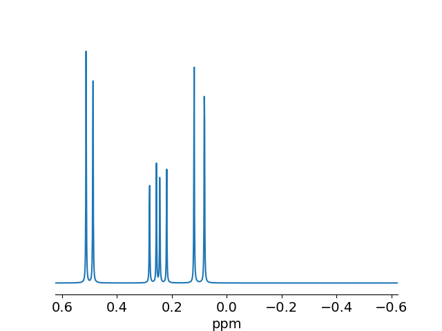
An example of simulating a single pulse experiment using pygamma.

import nmrglue as ng
import pygamma as pg

import matplotlib.pyplot as plt


sys = pg.spin_system()     # define the system, read in
sys.read("cosy1.sys") # from disk

print( sys)

dt2 = 0.002 # t2 time increment
t2pts = 1024 # points on t2 axis

udic = {'ndim': 1,
         0: { 'sw': 1/dt2,
              'dw': dt2,
              'complex': True,
              'obs': 400.0,
              'car': 0,
              'size': t2pts,
              'label': '1H',
              'encoding': 'direct',
              'time': False,
              'freq': True
            }
        }

fid = pg.row_vector(t2pts)      #block_1D tmp(t2pts); // 1D-data block storage

H = pg.Hcs(sys)+ pg.HJw(sys)             # // Hamiltonian, weak coupling
detect = pg.gen_op(pg.Fp(sys))     # // F+ for detection operator

sigma0 = pg.sigma_eq(sys)                      # // equilibrium density matrix
sigma1 = pg.Iypuls(sys, sigma0, 90)
pg.FID(sigma1,detect,H,dt2,t2pts,fid)

pg.exponential_multiply(fid,-5)
spec = fid.FFT()

npspec = spec.toNParray()

uc0 = ng.fileiobase.unit_conversion(udic[0]['size'],
                                     udic[0]['complex'],
                                     udic[0]['sw'],
                                     udic[0]['obs'],
                                     udic[0]['car'])

Out:

Spin Index :      0            1            2
Isotope    :      1H           1H           1H
Momentum   :     1/2          1/2          1/2
Shifts     :     0.00 Hz      0.00 Hz      0.00 Hz
           :     0.50 ppm     0.25 ppm     0.10 ppm
Js Spin 0  :                 10.00 Hz      0.00 Hz
Js Spin 1  :                              15.00 Hz
Omega      :   400.00 MHz   400.00 MHz   400.00 MHz

Plot 1D spectrum

plt.plot(uc0.ppm_scale(), npspec.real)
plt.xlim(uc0.ppm_limits())
plt.xlabel('ppm', fontsize=14)
plt.yticks([])
ax = plt.gca()
ax.spines['top'].set_visible(False)
ax.spines['left'].set_visible(False)
ax.spines['right'].set_visible(False)
ax.tick_params(axis='both', which='major', labelsize=14)