CSA Histogram Approach

Static Chemical Shift Powder Pattern using a Histogram Approach

The equation for the static powder pattern for a simple chemical shift anisotropy interation is given by the following equation

\[H = \delta_{iso} + \frac {1}{2} \delta \left ( 3 \cos^2 \theta - 1 \right ) - \delta \eta \sin^2 \theta \cos 2 \phi\]

There are a number of conventions for the assignment of \(\eta\) and \(\delta\), we have used Haeberlen’s convention.

if \(\sigma_{xx}\), \(\sigma_{yy}\) and \(\sigma_{zz}\) are the principal components of the chemical shielding tensor then they must have the following order.

\[\left | \sigma_{zz} - \sigma_{iso} \right | \ge \left | \sigma_{xx} - \sigma_{iso} \right | \ge \left | \sigma_{yy} - \sigma_{iso} \right |\]

where

\[\sigma_{iso} = \frac {1}{3} \left ( \sigma_{xx} + \sigma_{yy} + \sigma_{zz} \right )\]

and then \(\delta\) and \(\eta\) ared defined as follows

\[\delta = \sigma_{zz} - \sigma_{iso}\]

and

\[\eta = \frac {\sigma_{xx}-\sigma_{yy}}{\sigma_{zz}-\sigma_{iso}}\]

References

• 21. Haeberlen, In Advances in Magnetic Resonance; Suppl. 1; J. S. Waugh, Ed.; Academic Press, New York, 1976.

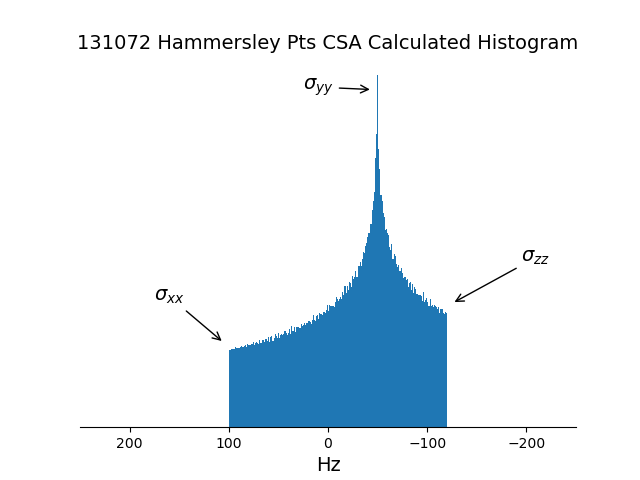
Out:

C:\Users\ERIC\Documents\pygamma_gallery\docsource\sphinx\examples\hammersleypoints\plot_csa_static_hist.py:159: UserWarning: Matplotlib is currently using agg, which is a non-GUI backend, so cannot show the figure.
  plt.show()

import numpy as np
from matplotlib import pyplot as plt
import sys


def return_Hammersley_points_array( l, n, p):
    """
    l is the power of x to go out to p^m
    n is the maximun number of points
    p is the order of the Hammersley point, 1,2,3,4,... etc

    returns
    --------
    np.array of double

    """

    vvv = np.zeros(n)

    for m in range(n):
        m1=1*m
        if p == 1:
            vvv[m] =  m1/n
        else:
            v = 0.0

            for j in range(l,-1,-1):
                num = m1//p**j

                if num > 0:
                    m1 -= num*p**j
                    v  += num / ( p ** (j+1) )

            vvv[m]=v

    return(vvv)


def omega_cs( theta, phi, iso_cs=0.0, asymm_cs=100, eta_cs=1.0):

    return (iso_cs +0.5* asymm_cs*(3.0 * (np.cos(theta)**2) -1.0 - eta_cs*(np.sin(theta)**2)*np.cos( 2.0 * phi ))), np.sin(theta)


if __name__ == "__main__":

    # Define CSA powder pattern

    # Principal components of the chemical shift shielding tensor

    s_zz = -120.0
    s_yy = -50.0
    s_xx =  100.0

    # Check for Haeberlens convention

    iso_cs =(s_zz+s_yy+s_xx)/3.

    if abs(s_zz-iso_cs) >= abs(s_xx-iso_cs) and abs(s_xx-iso_cs) >= abs(s_yy-iso_cs):
        h_zz = s_zz
        h_yy = s_yy
        h_xx = s_xx

    elif abs(s_zz-iso_cs) < abs(s_xx-iso_cs) and abs(s_xx-iso_cs) >= abs(s_yy-iso_cs):
        h_zz = s_xx
        h_yy = s_yy
        h_xx = s_zz

    else:
        print("problem with assignment of cs tensors")
        sys.exit()

    asymm_cs = h_zz-iso_cs
    eta_cs   = (h_xx-h_yy)/(h_zz-iso_cs)

    # Calculate Hammersley Points and Powder pattern
    N_particles = 2**17

    theta = return_Hammersley_points_array(22, N_particles, 2)
    phi   = return_Hammersley_points_array(22, N_particles, 3)

    omega, solid_angle = omega_cs(theta*np.pi,2*np.pi*phi, eta_cs=eta_cs, iso_cs=iso_cs, asymm_cs=asymm_cs)

    # Plot Powder pattern and use sin(theta) solid angle weighting

    plt.hist(omega, bins = 200, weights=solid_angle, density=True);
    plt.xlim(250.0, -250.0)
    ax = plt.gca()
    ax.spines['top'].set_visible(False)
    ax.spines['left'].set_visible(False)
    ax.spines['right'].set_visible(False)
    plt.yticks([])
    plt.xlabel('Hz', fontsize=14)

    ax.annotate('$\sigma_{xx}$',
            xy=(s_xx+5, 0.0030), xycoords='data',
            xytext=(-50, 30), textcoords='offset points',
            arrowprops=dict(arrowstyle="->"),fontsize=14)

    ax.annotate('$\sigma_{yy}$',
            xy=(s_yy+5, 0.012), xycoords='data',
            xytext=(-50, 00), textcoords='offset points',
            arrowprops=dict(arrowstyle="->"),fontsize=14)

    ax.annotate('$\sigma_{zz}$',
            xy=(s_zz-5, 0.0044), xycoords='data',
            xytext=(50, 30), textcoords='offset points',
            arrowprops=dict(arrowstyle="->"),fontsize=14)

    plt.title(f"{N_particles} Hammersley Pts CSA Calculated Histogram", fontsize=14);

    plt.show()